When to Retrain a Machine Learning Model
Machine learning models are rarely a case of “train once, deploy forever.” In production, the data often changes over time. This is true at Cash App, where the customer base and other actors will change their behavior, and it is especially true for Risk use cases, given the adversarial nature of identifying bad activity. The same challenge holds across nearly every industrial ML deployment. Therefore, many companies using AI to make predictions face the same issue: yesterday’s model might not work as well tomorrow.
However, retraining isn’t free. It costs compute, time, and human resources.
So how do you know when it’s actually worth retraining?
This blog post summarizes our method that answers this question.
The Real-World Dilemma
In a nutshell, the issue is that machine learning models are expensive to retrain, but letting performance degrade can be even more costly.
This sets up a tradeoff:
Retraining too often wastes resources (cost of retraining).
Retraining too rarely hurts performance (cumulative cost of low accuracy/false positives).
$\rightarrow$ We are looking for a retraining schedule that minimizes these two competing costs.
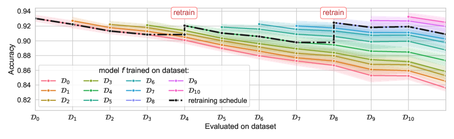
The problem can be visualized in the figure above. Each colored line represents the gradually decreasing performance of a model that was trained at a timestep (here, performance is measured by accuracy). The task is to determine when retraining is beneficial compared to keeping an older model. In the retraining schedule shown here, retraining occurs twice, at $\textstyle t = 4$ and $\textstyle t = 8$.
A Mathematical Formulation
To solve that problem, we introduce the following notation:
-
$pe_{i,j} = E[\ell (f_{i}(X_j), Y_j)]$ — the expected loss at time $j$ of a model trained at time $i$.
-
$\alpha$: cost-to-performance ratio set by the practitioner — i.e., how many dollars one percentage point of accuracy is worth at a timestep.
-
The vector $\boldsymbol{\theta} = [0, 0, 1, \dots]$ encodes a retraining schedule over a horizon $T$. For example, $\boldsymbol{\theta} = [0, 0, 1, 0, \dots] = [\text{wait}, \text{wait}, \text{retrain}, \text{wait}, \dots]$.
Target Objective
With this in hand, we can formulate the quantity to be minimized — the true cost of a retraining schedule $C_{\alpha}(\boldsymbol{\theta})$:
\[C_{\alpha}(\boldsymbol{\theta}) = \underbrace{\alpha \| \boldsymbol{\theta} \|_1}_{\text{cost of retraining}} + \underbrace{\sum\nolimits_{t=1\dots T} pe_{r_{\boldsymbol{\theta}}(t), t}}_{\text{cumulative cost of poor performance}}\]Finding the Right Retraining Schedule with UPF
Our solution is based on the realization that the only unknown in this equation is the future performance of models:
\[\tilde{C}_{\alpha}(\boldsymbol{\theta}) = \underbrace{ \color{gray} {\alpha \| \boldsymbol{\theta} \|_1}}_{\text{known}} + \underbrace{\color{orange} { \sum\nolimits_{t=1\dots T} pe_{r_{\boldsymbol{\theta}}(t), t}}}_{\text{unknown}}\]Our proposed Uncertainty-Performance Forecaster (UPF) method is based on two steps:
- Forecast probabilistic future model performance using a model trained on past model performances.
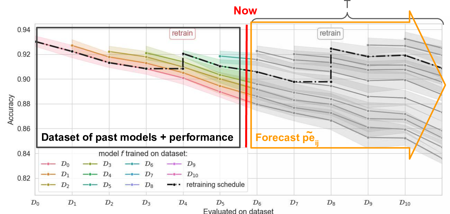
- Use the probabilistic forecast to make retraining decisions using a risk-averse criterion (based on a high-confidence quantile of the estimated cost).
We retrain or not by comparing the $\delta$-quantiles of $\tilde{C}$:
\[{F^{-1}}_{\tilde{C}_{\boldsymbol{\theta}_{<t}} \mid \text{retrain}}(\delta) \quad \text{vs} \quad {F^{-1}}_{\tilde{C}_{\boldsymbol{\theta}_{<t}} \mid \text{keep}}(\delta)\]The online decision rule is chosen by making the steps that will minimize the expected cost:
-
If \({F^{-1}}_{\tilde{C}_{\boldsymbol{\theta}_{<t}} \mid \text{retrain}}(\delta) < {F^{-1}}_{\tilde{C}_{\boldsymbol{\theta}_{<t}} \mid \text{keep}}(\delta)\)
$\rightarrow$ We predict that the $\delta$-quantile of the cost of retraining is smaller than if we do not retrain, so we retrain. -
Otherwise, we don’t retrain.
Key Takeaways
- To use our method, you need a rough estimate of the trade-off ratio $\alpha$ and some historical records of past model performance.
- Probabilistic forecasting and risk-averse decision-making are central to the approach.
- If you’re an ML engineer managing a model in production, especially under tight compute or human supervision budgets, this method can help you decide when to retrain.
- Even with very little data, smart modeling can go a long way.
For More Details
This blog is based on our recent publication at the International Conference on Machine Learning (ICML 2025), and was a collaboration between members of the Risk ML team — Florence Regol, Kyle Sprague, and Thomas Markovich — and academic contributors: Leo Schwinn from the Technical University of Munich (TUM) and Prof. Mark Coates from McGill University and MILA.