Friend Suggestions At Cash App

At Cash App, customers can invite their friends to join the platform and be rewarded for doing so. We built a ML model to populate a “Suggested Friends” section in the Invite Friends screen to help customers quickly find friends to invite without having to scroll through their whole contact book. In this post, we describe how we built it, the scalability issues we solved, and other things we learned along the way.

Introduction

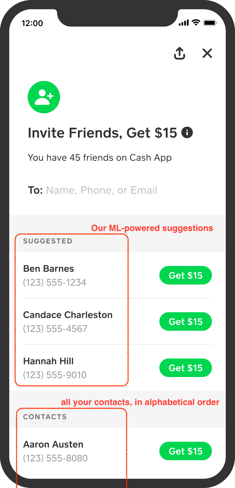
With Cash App, customers can easily send money to friends, family and businesses. These interactions form a social network of people (and merchants) transacting with each other, at a scale of 53 million monthly transacting actives (as of Q1 2023). As with many social networks, Cash App benefits from network effects: when people join Cash App, they often do so to specifically interact with others already there, and at the same time existing customers get more utility by having more of their friends in the network (for example, they can now avoid the hassle of carrying physical cash around, or of switching to another payment app). To lean on these network effects Cash App has a referral program, where a customer can be rewarded for inviting their friends (we typically offer between $5 and $15, some rules apply). To invite a friend, a customer goes to a specific page within the app; we will refer to it as “Invite Friends page” in this post. It currently looks like this:

At Cash App, consistent with our approach to privacy, we ask customers for permission to share their contact books with us. We do this to make it easy to find friends, protect their account, and prevent spam. Customers who decide to share their contact book benefit from the recommendation algorithm we discuss here.

The invitation flow consists of the following steps:

• select the friend(s) you want to invite
• send them a message with your referral code
• your friend (if they want) signs up for Cash App and enters the referral code in the process
• your friend then has 14 days to satisfy a few requirements (listed in our support page) and get paid.

If all goes well, you both receive some extra cash in your balance and you have one more friend you can transact with. Cash App has one more customer who in turn can invite new friends (possibly in a viral cascade). When blended with other marketing programs, invitations have helped Cash App acquire a new transacting active at an average cost of $10 or less and a less than one year payback (data from the 2022 investor day presentation).

If your contact book looks anything like mine, you’ll have your closest friends and family in there, coworkers, some extended family, some old friends from school or college, some acquaintances that you may not have talked to in years, a range of businesses you interact with (from small contractors to big retail chains), and probably people who you don’t even remember who they are.

Before we built the “suggested” section you can now see in the app, customers had to scroll through all of their contacts until they saw someone that they felt like inviting! In this project, we wanted to see if we could make it easier for customers to invite their friends, and we decided to build a section within the app to be populated with friends they might want to invite.

Good suggestions will result in more invitations and signups, while bad ones generally make for a bad customer experience (for example, being recommended friends that you don’t want to invite, or friends that don’t want to sign up for Cash App, meaning you will never get your reward).

As recommendations will never be perfect, we also wanted to make sure that the customer could still easily find their friends even when our system did not guess correctly. We currently show up to 3 suggestions, while your full contact book is still included just below in an easily scrollable alphabetical list.

Modeling

The problem that we set out to solve is the following: within your friends that are not yet on Cash App, who are you going to invite? Or more specifically, who are the top-3 friends you are most likely to invite?

First, let’s dive into the data: how can we predict who you are going to invite to Cash App, How can we do that, given that we know almost nothing about your friends or how close you are to them in real life? Because they are not on Cash App, the only thing we would know about them is that they are friends with you and other Cash App customers: for example, if many Cash App customers have one person in their contact book, they might be “at the edge” of the Cash App network, ready to be invited. But they might also not be interested in Cash App, or may have already been invited by other friends and consider any further invitation as spam from their friends: as this is a behavior we obviously don’t want to encourage, we include previous invitations history in the training data to help the model learn to not suggest these friends.

Let’s further frame the question as an ML problem:

• because the goal is to rank more relevant items first, this is a ranking problem, but can be treated as a classification step followed by a ranking step (a.k.a. pointwise ranking), meaning any binary classifier framework can be used in the first step. We chose to use a Gradient Boosting Decision Tree model (in particular, LightGBM) because of the great balance of speed, size and predictive power.
• our training dataset will be formed of (customer, friend) pairs, labeled as positive samples when the friend was invited (over a given time period) and negative otherwise. For each pair, we define features and train the model so it will predict the probability that the customer will invite that friend. In the ranking step, we then select the highest-scored friends to recommend to each customer.
• because customers don’t typically invite too many friends at once, the problem is an unbalanced one, but not massively so (imagine a few contacts invited over a few hundred entries in your contact book, resulting in a percent-level class imbalance).
• as opposed to many other recommendations problems, candidates are limited from the start (it’s just the friends you already have in your contact book) so we don’t need a candidate generation step to make the search space manageable in the reranking step.
• there are many ranking metrics, but we decided to focus on recall at k (the fraction of invited friends appearing in the top-k scored items) as the primary metric for recommendation quality, with mean average precision at k and overall invitation engagement metrics as guardrail metrics.

For each (customer, friend) pair in our dataset, we calculate many features which fall into three different categories (for most of these, we use our homegrown feature service, Blizzard, as described in a previous post in this blog to quickly define hundreds of features):

• many features about the customer sending the invite, e.g. how they are using Cash App, how active they are, how many friends they have invited, etc. By themselves, these would indicate the likelihood of a customer to invite anyone.
• a few features about the friend receiving the invite, e.g. how many people already on Cash App have them as friends, invitations previously received, etc. By themselves, these would indicate the likelihood of someone to be invited by anyone already on Cash App.
• then, some cross-product (customer, friend) features, e.g. previous invitations you already sent to that friend, or the number of friends on Cash App you and this friend have in common. These are the kind of features that are particularly important to predict if a given customer will invite a particular friend, as opposed to inviting anyone in general, or a friend being invited by anyone. In particular, we found that the “common friends” class of features is highly predictive but hard to compute for our problem: keep on reading to learn more about how we calculated these features at scale!

Features - Common Friends

What does it mean to have friends in common with someone? For example, take the following sentence:

You and your friend have 2 common friends on Cash App

This means that two of your friends who are on Cash App are also friends of this person. If you have many friends in common with someone, it is more likely that you are closely connected to them in the real world (your friendship “circles” overlap more). Furthermore, because many of their friends are already here, they also have more reasons to join Cash App and your invite (and the reward!) might be the one that convinces them to finally join.

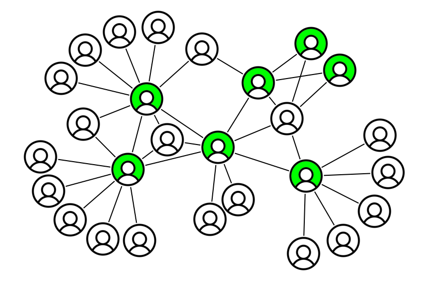
Let’s take a look at what a sample friendship graph might look like:

Mathematically, given a node \(x\) let’s call \(\Gamma(x)\) its one-hop neighborhood for a given edge class (the set of edges associated to the node) and \(k(x) = \vert\Gamma(x)\vert\) its degree (the number of edges associated to the node): the number of common friends between \(x\) and \(y\) is then just \(\vert\Gamma(x) \bigcap \Gamma(y)\vert\). There are many other metrics based on the intersection of one-hop neighborhoods, such as cosine similarity, Jaccard index, Adamic-Adar index and so on (e.g. see this non-exhaustive list). As they mostly just differ by normalization factors, in this post we will focus on the common friends feature, but the generalization is straightforward.

While we have drawn a simple graph above, there are multiple ways people can connect with each other. In graph theory language, this forms a heterogeneous graph, defined by:

• nodes representing people, which can be customers (shaded in green) or non-customers (just in white). In this problem, friends that can be invited are currently non-customers, but the moment they sign up they become customers; in this case, it is best to treat all nodes as a homogeneous class (same type of node).
• edges representing friendship between people, which can be defined in multiple ways (and directions):
  • being in someone’s contact book, having them in your contact book, or either
  • paying a friend with Cash App, receiving money from them, or either
  • having previously invited a friend to join Cash App (in fact, this type of link is exactly what we are trying to predict, for the future)

The heterogeneous edge classes in this graph have different cardinalities and will overlap only partially: for example, you might have friends in your contact book that you’ve never interacted with in the app (it might even be most of them!), or friends not in your contact book that you interact with a lot on Cash App. These different types of edges allow us to define different kinds of “common friends” features: for example, “p2p common friends” would be friends that you’ve sent money to that also have your not-on-cash-app friend in their contact book. There is also a time component on both nodes and edges, meaning we can calculate features like “recently added common friends”, or “most frequently paid common friends”. To simplify the discussion, in this post we only consider one class of undirected edges.

Operationally, calculating the number of common friends between you and your friend means counting the number of triangles that have you and your friend as one of the edges. For example, let’s zoom in into a given customer in the above graph:

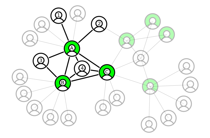
Let’s pick customer A and examine a few (customer, friend) pairs:

• (A, 1) have zero common friends, because node 1 is disconnected from any other node
• (A, 2) have zero common friends, because even though node 2 is connected to another customer, that customer is not friends with A (in fact, they are two hops away).
• (A, 3) have one common friend, because they are connected to customer B who is friends with A.
• (A, 4) have two common friends, customers B and C who are both friends of A.

In this example of an undirected graph, the calculation is symmetric, e.g. if B is a common friend of (A, 3) then A is a common friend of (B, 3), but this would not always be the case if we considered directional edges. In addition to directionality, heterogeneous edges and weighing nodes based on their features allows us to maximize the information extracted from the graph.

But what does it mean to compute the “number of triangles”? If the graph edges form a table graph with (source, destination) columns (this assumes directionality of the edges, but can be easily tweaked to remove the direction), we would use the following SQL query:

select t1.source
, t1.destination
, count(t3.destination) as count_common_friends
from graph as t1
join graph as t2
 on t1.source = t2.source
join graph as t3
 on t3.source = t2.destination
   and t3.destination = t1.destination
where is_cash_customer(t1.source)
  and is_not_cash_customer(t1.destination)
  and is_cash_customer(t2.destination)
group by t1.source, t1.destination

Inspecting the query, for a given origin \(s_0\) the first self-join creates node pairs \((x_i, x_j)\), while the second one closes the triangle when such an edge exists between these pairs. The where filter is because we are only interested in (customer, non-customer) pairs as for the problem at hand (calculating this feature for friends not yet on Cash). Finally, we aggregate by the (source, destination) link and count the number of entries, which is the number of friends.

Let’s run through the logic for the example customer A and the highlighted nodes in the graph above:

• the 1-hop neighborhood of A is given by the nodes [1, 2, 3, 4, B, C].
• there are 15 distinct candidate pairs in this one-hop neighborhood (simply combinations([1, 2, 3, 4, B, C], 2)), of which only 8 (customer, non-customer) pairs (2 “on cash” nodes * 4 “not on cash” nodes), marked in the center figure as gray lines with a question mark.
• we then filter the candidate pairs to the ones for which an edge actually exists in the graph and count the number of connections for a given alias, yielding one common friend for node 3, two common friends for node 4, and zero for all other nodes.
• note that in the second step we pre-filtered the candidate pairs to (customer, non-customer) pairs that have a chance of actually being connected: for example, the triangle (A, 1, 2) cannot exist as there is no (1, 2) edge between nodes that are not on Cash App, and while the triangle (A, B, C) exists it is not useful to count common friends between A and friends to be invited to Cash App).

Computationally, because we are going two hops away from a node before returning to it on the final edge, if \(\langle k \rangle\) is the average node degree, we generate \(\langle k \rangle^2\) candidate pairs before being able to check for the final edge. For a typical contact book with hundreds of contacts, this generates tens of thousands of candidate pairs (even only generating distinct pairs with exactly one Cash App customer in them, the O(n) analysis is the same). With this calculation repeated over 50 millions monthly actives (Cash App’s scale), we would generate on the order of trillions of candidate pairs; more than could be computed at reasonable cost or speed.

While parallelizing the calculation at the customer level by partitioning the graph used in the first two hops is possible (and is how we computed this feature on our smaller training data), it was not an effective solution for the full population, as the two-hop candidate pairs typically span multiple partitions - we still would need to load and join the full graph to close the last edge.

Common Friends Calculation at Scale

To solve this problem at scale, we used sampling techniques inspired by the paper “Dimension Independent Similarity Computation” by Zadeh and Goel to compute pairwise similarities. We sample nodes and edges to reduce the computational complexity of the problem to a fixed, manageable scale, at the cost of introducing some approximation error which can be evaluated during model training (comparing model performance using the exact and approximate values with different hyperparameters choices). Let’s walk through the same example graph we just discussed while detailing the algorithm as we implemented it:

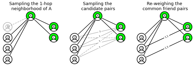
• to reduce the negative impact of high-degree nodes, we take a max node size \(K_0\) and for nodes with \(k>K_0\), we sample edges with a probability \(K_0/k(x)\). On average, this reduces the node degree from \(\langle k \rangle\) to \(K_0\), and particularly helps with reducing the disproportionate effect of high-degree outliers.
  • in the example graph, we set \(K_0 = 5\), and drop one node from the neighborhood of A (note that this will also thin out the neighborhoods of nodes B, C, not shown here)
• next, instead of generating all candidate pairs \((x, y)\), we sample them with probability \(P(x, y) = \frac{F}{\sqrt{k(x)k(y)}}\), where F is a constant: this drops edges connected to “large” nodes and in average, reduces the number of generated pairs from \({K_0}^2\) to \(F\).
  • in the example, we set \(F=3\) and from the candidate pairs on the remaining graph (note that node 1 was already dropped from consideration) we drop two edges due to random sampling with probability \(P(x, y)\) which penalizes edges between high degree nodes.
• Finally, we count the number of common friends on the remaining graph. As we have reduced the number of pairs generated, obviously the count in the sampled graph will be lower than the real number of common friends (with the above probability, the sampling discussed in the above paper would actually compute the cosine similarity between the 1-hop neighborhoods). To make up for this, we re-weigh the surviving pairs by the inverse of the sampling probability, \(1/P(x, y)\) (in average, removing the effect of the previous sampling) and get an approximate count that in average matches the common friend count.
  • in the example, we weigh each remaining pair by the inverse of the sampling probability, meaning we get an approximate count of common friends equal to 1.1 for node 3 and 1.3 for node 4. Compared to the exact values of 1 and 2, this is directionally correct, with the large approximation error due to the small sample size and small hyperparameters used.

To get an idea of how this approach helps in a more realistic case, let’s plug in some numbers: if the average contact book has 200 entries, choosing \(K_0=100\) (sampling half of contacts in each book), would reduce the number of candidate pairs from 40k to 10k (a 4x improvement), and then choosing \(F=1000\) (sampling 1k of these 10k pairs), we would reduce the size of the problem by an overall factor of 40! Of course, as edges and nodes are dropped some information is lost: the sampling factors are hyperparameters of the algorithm and should be tuned depending on the properties of the graph (degree, connectedness, …) and the acceptable loss in predictive power. In our case, we were able to achieve almost equal model performance using this technique, while accelerating feature calculation from what would have been days to a few hours.

Conclusions

Finally, building a model is only a fraction of the work to be done in order to impact customers, especially as this was the first time we computed and showed this type of recommendations. We also worked with our ML engineering teams to serve model predictions online, with our client engineers to show the recommendations in Cash App, and with our product data scientists to design and execute A/B tests to measure the impact of recommendations on our top-line metrics. After measuring statistically significant lifts in invitations, we rolled out the feature to all customers, and have since been monitoring recommendations quality and how customers use them.

In the Personalization ML team, we will keep exploring opportunities to improve recommendations, iterating on signals and models with an eye on our long-term goal to make it easy for everyone to connect on Cash App.

If you’re interested in this type of problems or you have feedback for this post, feel free to contact me at angelo@squareup.com.